Actuarial notation

Actuarial notation is a shorthand method to allow actuaries to record mathematical formulas that deal with interest rates and life tables.

Traditional notation uses a halo system where symbols are placed as superscript or subscript before or after the main letter. Example notation using the halo system can be seen below.

Various proposals have been made to adopt a linear system where all the notation would be on a single line without the use of superscripts or subscripts. Such a method would be useful for computing where representation of the halo system can be extremely difficult. However, a standard linear system has yet to emerge.

1 Example notation
2 Force of mortality
3 See also
4 External links

Example notation

Interest rates

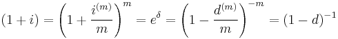
$\,i\!$ is the annual effective interest rate, which is the "true" rate of interest over a year. Thus if the annual interest rate is 12% then $\,i = 0.12\!$ .

$\,i^{(m)}\!$ is the nominal interest rate convertible $m$ times a year, and is numerically equal to $m$ times the effective rate of interest over one $m$ ^th of a year. For example, $\,i^{(2)}\!$ is the nominal rate of interest convertible semiannually. For example, if the effective annual rate of interest is 12%, then $\,i^{(2)}/2\!$ represents the effective interest rate every six months. Since $\,(1.0583)^{2}=1.12\!$ , we have $\,i^{(2)}/2=0.0583\!$ and hence $\,i^{(2)}=0.1166\!$ . The ^"(n)" appearing in the symbol $\,i^{(n)}\!$ is not an "exponent." It merely represents the number of interest conversions, or compounding times, per year. Semi-annual compounding, (or converting interest every six months), is frequently used in valuing bonds (see also fixed income securities) and similar monetary financial liability instruments, whereas home mortgages frequently convert interest monthly. Following the above example again where $\,i=0.12\!$ , we have $\,i^{(12)}=0.1139\!$ since $\,(1%2B\frac{0.1139}{12})^{12}=1.12\!$ .

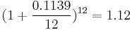Effective and nominal rates of interest are not the same because interest paid in earlier measurement periods "earn" interest on interest in later measurement periods; which is called compound interest. That is, nominal rates of interest credit interest to an investor, (alternatively charge, or debit, interest to a debtor), more frequently than do effective rates. The result is more frequent compounding of interest income to the investor, (or interest expense to the debtor), when nominal rates are used.

$\,v\!$ is the present value of 1 at interest rate i or discount factor over a year, (since it is multiplied by an amount of money one year in the future to obtain the value of this aforementioned amount today); that is, it can be obtained from $\,v = {(1%2Bi)}^{-1}\!$ . A discount factor is used to obtain the amount of money that must be invested now in order to have a given amount of money in the future. For example if you need 1 in one year then the amount of money you need now is: $\,1 \times v\!$ . If you need 25 in 5 years the amount of money you need now is: $\,25 \times v^5\!$ .

Alternatively, the discount factor is the factor that should be multiplied with the amount one year from now so as to discount to the present value of that amount.

$\,d\!$ is the annual effective discount rate. From $\,(1-d) = v = {(1%2Bi)}^{-1}\!$ , the rate of discount is computed by reference to a balance of money at the end of a measurement period, (but paid or accrued at the beginning of a measurement period), which is in contrast to a rate of interest which is calculated by reference to a balance of money at the beginning of a measurement period, (but paid or accrued at the end of a measurement period). The rate of interest - the present value of 1 now, evaluated $\,n$ years before, is $\,{(1-d)}^{n}\!$ , which is analogous to the formula $\,{(1%2Bi)}^{n}\!$ for present value evaluated $\,n$ years later.

$\,d^{(m)}\!$ , the nominal rate of discount convertible $\,m\!$ times a year, is analogous to $\,i^{(m)}\!$ . Discount is converted on an $m$ ^th-ly basis.

$\,\delta\!$ , the force of interest, is the limiting value of the nominal rate of interest when $m$ increases without bound:

In this case, interest is convertible continuously.

The general relationship between $\,i\!$ , $\,\delta\!$ and $\,d\!$ is:

And their numerical value is compared as follows:

Life tables

A life table (or a mortality table) is a mathematical construction that shows the number of people alive (based on the assumptions used to build the table) at a given age, or other probabilities associated with such a construct.

$\,l_x\!$ is the number of people alive, relative to an original cohort, at age $x$ . As age increases the number of people alive decreases.

$\,l_0\!$ is starting point: the number of people alive at age 0. This is known as the radix of the table.

$\omega\!$ is the limiting age of the mortality tables. $\,l_n\!$ is zero for all $\,n \geq \omega\!$ .

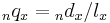
$\,d_x\!$ shows the number of people who die between age $x$ and age $x %2B 1$ . You can calculate $\,d_x\!$ using the formula $\,d_x = l_x - l_{x%2B1}\!$

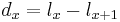
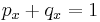
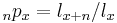
$\,q_x\!$ is the probability of death between the ages of $x$ and age $x %2B 1$ .

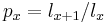
$\,p_x\!$ is the probability of a life age $x$ surviving to age $x %2B 1$ .

Since the only possible alternatives from one year (age $x$ ) to the next (age $x%2B1$ ) are living or dying, the relationship between these two probabilities is:

These symbols also extend to multiple years, by adding the number of years at the bottom left of the basic symbol.

$\,_nd_x = d_x %2B d_{x%2B1} %2B \cdots %2B d_{x%2Bn-1} = l_x - l_{x%2Bn}\!$ shows the number of people who die between age $x$ and age $x %2B n$ .

$\,_nq_x\!$ is the probability of death between the ages of $x$ and age $x %2B n$ .

$\,_np_x\!$ is the probability of a life age $x$ surviving to age $x %2B n$ .

An important information that can be obtained from the life table is the life expectancy.

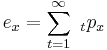
$\,e_x\!$ is the curtate expectation of life for the people alive at age $x$ . This is the expected number of complete years remaining to live (you may think of it as the number of birthdays they will celebrate).

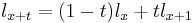
A life table generally shows the number of people alive at integral ages. If we need information regarding a fraction of a year, we must make assumptions with respect to the table, if not already implied by a mathematical formula underlying the table. A common assumption is that of a Uniform Distribution of Deaths (UDD) at each year of age. Under this assumption, $\,l_{x%2Bt}\!$ is a linear interpolation between $\,l_x\!$ and $\,l_{x%2B1}\!$ . i.e.

Annuities

The basic symbol for the present value of an annuity is $\,a\!$ . The following notation can then be added:

Notation to the top-right indicates the frequency of payment. A lack of notation means payments are made annually.
Notation to the bottom-right indicates the age of the person when the annuity starts and the period for which an annuity is paid.
Notation directly above indicates when payments are made. Two dots indicates an annuity payable at the start of the year, a horizontal line indicates an annuity payable continuously, whilst nothing indicates an annuity payable at the end of the year.

If the payment period of an annuity is independent of any life event, this is known as an annuity-certain. Otherwise, in particular if payments end on the beneficiary's death, it is called a life annuity.

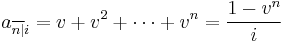
$a_{\overline{n|}i}$ (read a-angle-n-at i) represents the present value of an annuity-immediate, which is a series of unit payments at the end of each year for $n$ years (in other words: the value one period before the first of n payments). This value is obtained from:

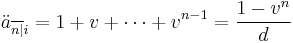
$\ddot{a}_{\overline{n|}i}$ represents the present value of an annuity-due, which is a series of unit payments at the beginning of each year for $n$ years (in other words: the value at the time of the first of n payments). This value is obtained from:

$\,s_{\overline{n|}i}$ is the value at the time of the last payment, $\ddot{s}_{\overline{n|}i}$ the value one period later.

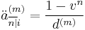
If the symbol $\,(m)$ is added to the top-right corner, it represents the present value of an annuity whose payment of is made every one $m$ ^th of a year for a total number of $n$ years, and each payment is one $m$ ^th of a unit.

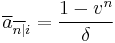
$\overline{a}_{\overline{n|}i}$ is the limiting value of $\,a_{\overline{n|}i}^{(m)}$ when $m$ increases without bound. The underlying annuity is known as a continuous annuity.

The present value of these annuities are compared as follows:

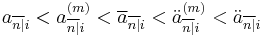
because cash flows at later time has a smaller present value compared with the cash flows of the same size but at earlier time.

The subscript $i$ which represents the rate of interest may be replaced by $d$ or $\delta$ , and is often omitted if the rate is clearly known under the context.
When using these symbols, the rate of interest is not necessarily constant throughout the lifetime of the annuities. However, when the rate varies, the above formulas will not longer be valid, and particular formulas can be developed for particular movements of the rate.

Life annuities

Life annuities are those contingent on the death of the annuitant. The age of the annuitant is important information when we want to calculate the actuarial present value of the annuities.

The age of the annuitant is put at the bottom-right, without the "angle".

For example:

$\,a_{65}\!$ indicates an annuity of 1 unit per year payable at the end of each year until death to someone currently age 65

$a_{\overline{10|}}$ indicates an annuity of 1 unit per year payable for 10 years with payments being made at the end of the year

$a_{65:\overline{10|}}$ indicates an annuity of 1 unit per year for 10 years, or until death if earlier, to someone currently age 65

$a_{65}^{(12)}$ indicates an annuity of 1 unit per year payable 12 times a year (1/12 unit per month) until death to someone currently age 65

${\ddot{a}}_{65}$ indicates an annuity of 1 unit per year payable at the start of each year until death to someone currently age 65

or in general:

$a_{x:\overline{n|}i}^{(m)}$ , where $x$ is the age of the annuitant, $n$ is the number of years of guaranteed payments, and $m$ is the number of payments per year, and $i$ is the interest rate.

In the interest of simplicity the notation is limited and cannot show:

Whether the annuity is payable to a man or a woman
The Actuarial Present Value of life contingent payments can be treated as the mathematical expectation of the present value random variable, or calculated through the current payment form.

Life insurance

The basic symbol for life insurance is $\,A\!$ . The following notation can then be added:

Notation to the top-right indicates the timing of death payment. A lack of notation means payments are made at the end of the year of death. A figure in parenthesis (for example $A^{(12)}$ ) means the benefit is payable at the end of the period indicated (12 for monthly; 4 for quarterly; 2 for semi-annually; 365 for daily).
Notation to the bottom-right indicates the age of the person when the life insurance begins.
Notation directly above indicates the "type" of life insurance, whether payable at the end of the period or immediately. A horizontal line indicates life insurance payable immediately, whilst nothing indicates payment at the end of the period indicated.

For example:

$\,A_x\!$ indicates a life insurance benefit of 1 payable at the end of the year of death.

$\,A_x^{(12)}\!$ indicates a life insurance benefit of 1 payable at the end of the month of death.

$\,\overline{A}_x\!$ indicates a life insurance benefit of 1 payable at the (mathematical) instant of death.

Force of mortality

Among actuaries, force of mortality refers to what economists and other social scientists call the hazard rate and is construed as an instantaneous rate of mortality at a certain age measured on an annualized basis.

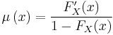
In a life table, we consider the probability of a person dying from age (x), that is, a person age x, to (x+1), a person age x + 1, called q_x. In the continuous case, we could also consider the conditional probability of a person, who attained age (x), dying from age (x) to age (x+Δx) as:

$P_{\Delta x}(x)=P(x<X<x%2B\Delta\;x\mid\;X>x)=\frac{F_X(x%2B\Delta\;x)-F_X(x)}{(1-F_X(x))}$

where F_X(x) is the distribution function of the continuous age-at-death random variable, X. As Δx tends to zero, so does this probability in the continuous case. The approximate force of mortality is this probability divided by Δx. If we let Δx tend to zero, we get the function for force of mortality, denoted as μ(x):